Variography as Fundamentals in Resource Estimation

When working with geological data, it’s not just about what numbers you have, it’s about how those numbers connect across space. That’s where variograms come in. They help us understand patterns hidden in data, making resource estimation more reliable. In this article, we’ll unpack what a variogram really is, show how it’s used in real mining scenarios, and explore how GEOVIA Surpac makes it easier to visualize and model spatial variability.

A. Get to Know Variogram in Geostatistic

Most geoscience data inherently have spatial continuity property (for example, ore grade data), that means if two data close to each other are more likely to have similar values than two data that are far apart (Isaaks and Srivastava, 1989). To know how similar or dissimilar the data is in a space, the conventional statistic cannot take into account this spatial correlation, thus we used geostatistics in order to measure spatial continuity. Variogram modelling is usually done after understanding the characteristic of data statistically (usually using EDA method) and can be used to gain the weighting factor in estimation functions like Ordinary Kriging and other advanced estimation methods.

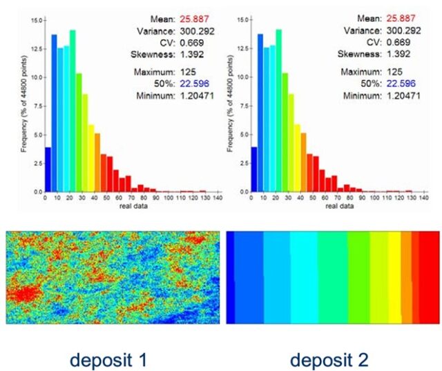
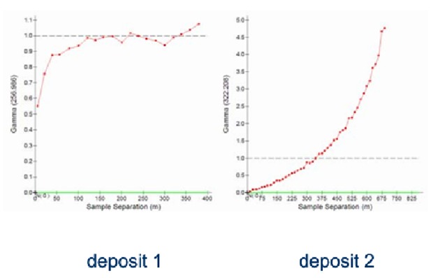
Examples of two deposit with same descriptive statistic properties, but have different spatial location (retrieved from Snowden, 2009)

Variogram and its part description (retrieved from GEOVIA Surpac Tutorial)

A variogram is created by plotting the average variability γ(h) for all sample pairs at a certain distance apart against that separation distance (h). It can be calculated either only based on the separation distance or by separation distance respected to a certain direction. When calculating variogram, the separation distance or/and direction vector or “h” (e.g. 10 m north-south). The average variability is calculated for a series of lags and plotted against lag distance to create a variogram plot.

The bigger the distance is, the higher the difference between samples that can be shown by the corresponding average variability increases in scatterplot until the total data variance when it reaches the peak, we called that point as sill. While the separation distance at which the sill is reached is called the range that indicates the distance there is no longer correlation between samples.

B. Calculating Variogram

A variogram can be calculated using the equation below (Isaak dan Srivastava, 1989):

Semivariance (Isaak dan Srivastava, 1989)

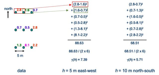
A variogram quantifies the spatial variability by taking half of the squared differences between paired sample values (v) divided by the sum of N(h) pairs that are separated by the same specific distance and direction. Essentially, it reflects the average dispersion or spread of the data points in the h-scatter plot for each lag interval.

Based on the equation above, the value of the variogram for h = 0 supposed to be 0, several factors, like sampling error and short distance variability, may cause a discontinuity as sample values separated by extremely small distances appear to be quite dissimilar. The vertical jump from 0 at h=0 is called the nugget effect.

For further understanding of the standar variogram calculation, pay attention to Figure 3 below.

Worked example – variogram calculation (retrieved from Snowden, 2009)

C. Variogram Modelling

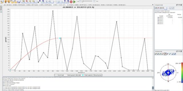
Today, variogram models are not only required for resource estimation as it is needed for the estimation calculation as the weighting factor but also as a tool to validate our domain orientation and spatial continuity. GEOVIA Surpac is one of the most robust software for geological 3D modelling for mining, and one of its robust tools is the capability to run geostatistic analysis, including variogram modelling.

1. Variogram type in GEOVIA Surpac

In calculating the variogram, we need to adjust the method of calculation used based on the data statistical distribution (Snowden, 2009). Here are some of the methods that supported in GEOVIA Surpac:

The Normalised variogram divides each gamma(h) by the variance of the data set. This gives a gamma(h) range between 0 and 1. Most effective for positively skewed distribution or can be applied for negatively skewed data.
The Standard variogram is calculated from untransformed data and is used as the basis of modelling. Works well for data with tiny or no skew or can be used for negatively skewed.
The Logarithmic variogram is calculated using the logarithms of the raw data and mitigates the effect of extreme values. While sills and nuggets cannot be derived from the logarithmic variogram, the range may be determined and it is possible that structures are more easily resolved
The General Relative variogram divides each gamma(h) by the squared mean of all samples used to estimate that gamma(h).
The Pairwise Relative variogram uses the square of the mean of each sample pair for each pair. As for the logarithmic variogram, units along the Y (gamma(h)) axis have no meaning but the relative variograms may serve to identify ranges and structures. Useful for domains containing a limited number of samples.

2. Parameters for variogram calculations in GEOVIA Surpac

In the first step after we prepared the composited domain data, we need to set the parameter in variogram modelling

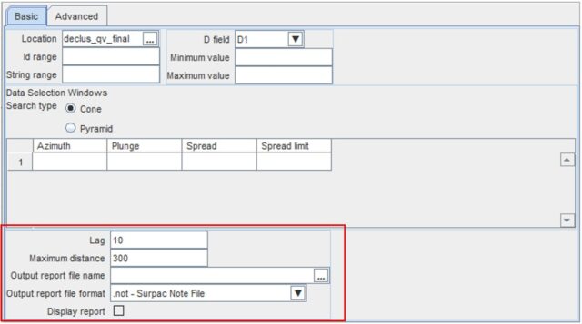
The window for importing and setting the parameter for variogram modelling in Surpac (red box)

Lag: Separation distance for sample pair selection. The variogram γ(h) is calculated at distances that are multiples of a chosen lag, up to a set maximum (e.g., 10 m). A tolerance of half the lag is used—for example, with a lag of 2, pairs between 1 and 3 units apart are included.
Max of distance: the maximum number of lags (e.g., 300)
Angle: this is an additional parameter if you are doing directional variogram. The angle of the direction of maximum continuity.

3. Model Types

The shape of the variability of nugget effect and the total sill is controlled by the variogram model type. In Surpac, there are four model types available

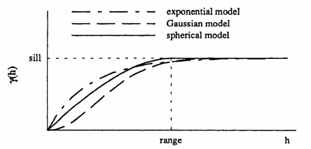
The three most commonly used variogram model (retrieved from Isaaks and Srivastava, 1989)

Spherical model linear for short separation distances and then curves into the sill near the range of influence.
Exponential model curves from zero separation distance until it levels off near the range of influence.
The Gaussian model has a flat almost nugget-like contribution for short distances, before it curves towards the sill in much the same way as the exponential model. This model suggests a degree of smoothing has occurred at short distances.
Hole Effect due to “banding” in the mineralisation and where there are repeated zones of mineralisation and waste. This banding manifests itself in the variogram as waves where the peaks indicate the distances of maximum difference and troughs indicate the separation distance for repeated similarity (Snowden, 2009).